Normal Probability Distribution

Solved Examples: Normal Distribution

Samuel Dominic Chukwuemeka (SamDom For Peace)

Prerequisite Topics
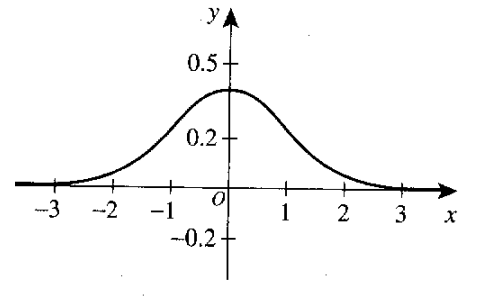
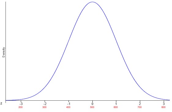
Probability Distribution Calculators
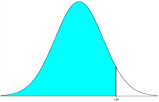
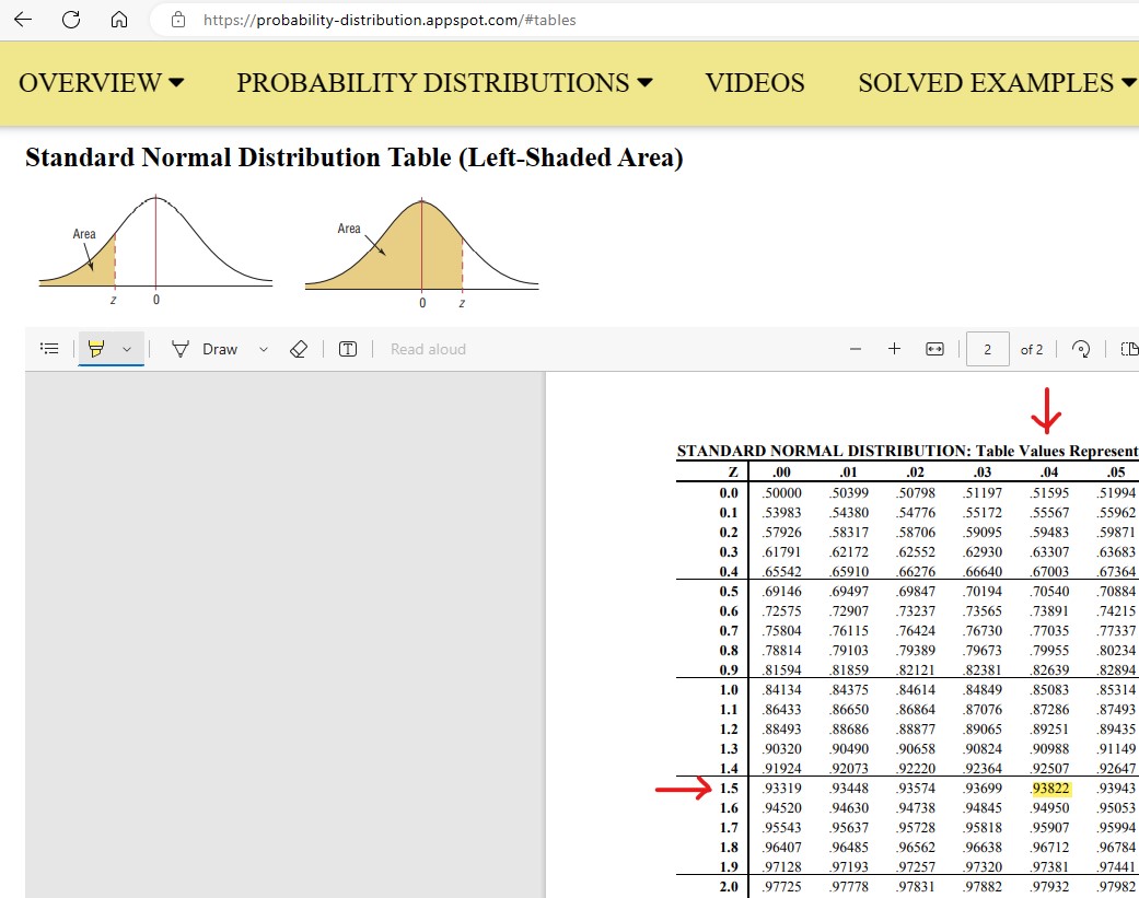
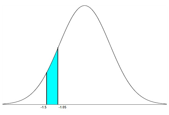
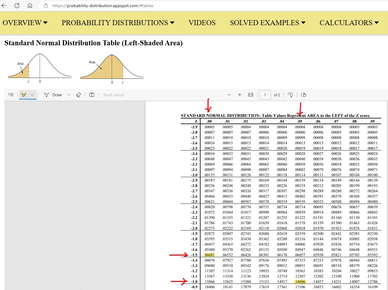
Normal Distribution Table (Left-Shaded Area)
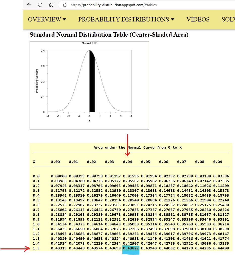
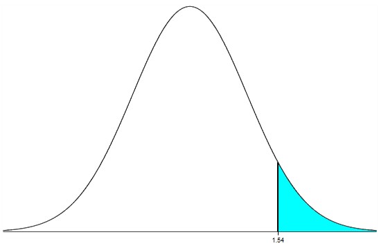
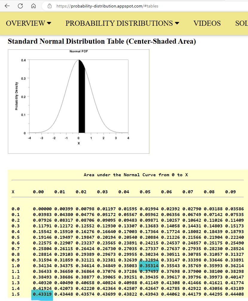
Normal Distribution Table (Center-Shaded Area)

For ACT Students
The ACT is a timed exam...$60$ questions for $60$ minutes
This implies that you have to solve each question in one minute.
Some questions will typically take less than a minute a solve.
Some questions will typically take more than a minute to solve.
The goal is to maximize your time. You use the time saved on those questions you solved in less than a minute, to solve the questions that will take more than a minute.
So, you should try to solve each question correctly and timely.
So, it is not just solving a question correctly, but solving it correctly on time.
Please ensure you attempt all ACT questions.
There is no negative penalty for any wrong answer.
Use the functions in your TI-84 Plus or TI-Nspire to solve some of the questions in order to save time.

For WASSCE Students
Any question labeled WASCCE is a question for the WASCCE General Mathematics
Any question labeled WASSCE-FM is a question for the WASSCE Further Mathematics/Elective Mathematics

For NSC Students
For the Questions:
Any space included in a number indicates a comma used to separate digits...separating multiples of three digits from behind.
Any comma included in a number indicates a decimal point.
For the Solutions:
Decimals are used appropriately rather than commas
Commas are used to separate digits appropriately.

Solve all questions.
Show all work.
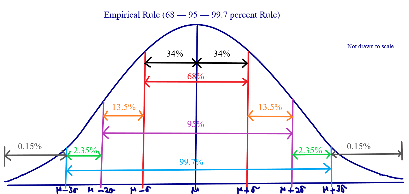
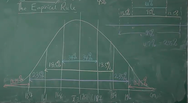
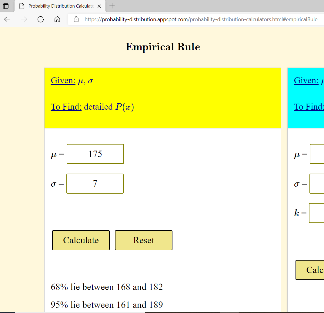
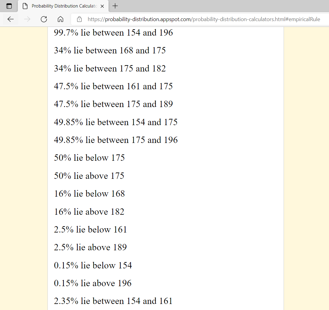
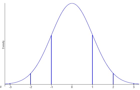
To accommodate all students, as applicable; use at least three methods to solve each question: Empirical Rule, Left-Shaded Area Table, and Center-Shaded Area Table.

(1.) The heights of the Golden State Warriors basketball team players have a bell-shaped distribution with mean of 175 cm and standard deviation of 7 cm.
(a.) Analyze this information using the Empirical Rule.

(b.) (i) Draw the normal distribution curve for the information.
(ii) Indicate the area of each region in the curve.

(c.) Verify the area of each region using the results from the appropriate section of the Probability Distribution calculators.

Treat the dataset as a sample
But you may choose to treat it as a population if you wish
(a.)
Empirical Rule $(68 - 95 - 99.7\%\;\;Rule)$

$ \bar{x} = 175\;cm \\[3ex] s = 7\;cm \\[3ex] 1s = 1(7) = 7\;cm \\[3ex] 2s = 2(7) = 14\;cm \\[3ex] 3s = 3(7) = 21\; cm \\[3ex] \underline{1\;standard\;\;deviation\;\;below\;\;the\;\;mean} \\[3ex] \bar{x} - 1s \\[3ex] 175 - 7 \\[3ex] 168\;cm \\[3ex] \underline{1\;standard\;\;deviation\;\;above\;\;the\;\;mean} \\[3ex] \bar{x} + 1s \\[3ex] 175 + 7 \\[3ex] 182\;cm \\[3ex] $ This impies that 68% of the basketball team players have heights between 168 cm and 182 cm

$ \underline{2\;standard\;\;deviations\;\;below\;\;the\;\;mean} \\[3ex] \bar{x} - 2s \\[3ex] 175 - 14 \\[3ex] 161\;cm \\[3ex] \underline{2\;standard\;\;deviations\;\;above\;\;the\;\;mean} \\[3ex] \bar{x} + 2s \\[3ex] 175 + 14 \\[3ex] 189\;cm \\[3ex] $ This impies that 95% of the basketball team players have heights between 161 cm and 189 cm

$ \underline{3\;standard\;\;deviations\;\;below\;\;the\;\;mean} \\[3ex] \bar{x} - 3s \\[3ex] 175 - 21 \\[3ex] 154\;cm \\[3ex] \underline{3\;standard\;\;deviations\;\;above\;\;the\;\;mean} \\[3ex] \bar{x} + 3s \\[3ex] 175 + 21 \\[3ex] 196\;cm \\[3ex] $ This impies that 99.7% of the basketball team players have heights between 154 cm and 196 cm

(b.) (i)
Number 1b

$ Center = \bar{x} = 175 \\[3ex] Between\;\;168\;\;and\;\;182 = 68\% \\[3ex] symmetrical \implies \\[3ex] Between\;\;168\;\;and\;\;175 = \dfrac{68}{2} = 34\% \\[5ex] Similarly:\;\;between\;\;175\;\;and\;\;182 = 34\% \\[3ex] Between\;\;161\;\;and\;\;189 = 95\% \\[3ex] symmetrical \implies \\[3ex] Between\;\;161\;\;and\;\;175 = \dfrac{95}{2} = 47.5\% \\[5ex] \implies \\[3ex] Between\;\;161\;\;and\;\;168 = 47.5 - 34 = 13.5\% \\[3ex] Similarly:\;\;between\;\;175\;\;and\;\;189 = 47.5\% \\[3ex] Similarly:\;\;between\;\;182\;\;and\;\;189 = 13.5\% \\[3ex] symmetrical \implies \\[3ex] Between\;\;154\;\;and\;\;196 = \dfrac{99.7}{2} = 49.85\% \\[5ex] \implies \\[3ex] Between\;\;154\;\;and\;\;161 = 49.85 - (34 + 13.5) = 49.85 - 47.5 = 2.35\% \\[3ex] Similarly:\;\;between\;\;175\;\;and\;\;196 = 49.85\% \\[3ex] Similarly:\;\;between\;\;189\;\;and\;\;196 = 2.35\% \\[3ex] Total\;\;area = 100\% \\[3ex] symmetrical \implies \\[3ex] \le 175 = \dfrac{100}{2} = 50\% \\[5ex] \ge 175 = \dfrac{100}{2} = 50\% \\[5ex] \implies \\[3ex] \lt 154 = 50 - (2.35 + 13.5 + 34) = 50 - 49.85 = 0.15\% \\[3ex] Similarly:\;\; \gt 196 = 0.15\% \\[3ex] \lt 161 = 2.35 + 0.15 = 2.5\% \\[3ex] Similarly:\;\; \gt 189 = 2.5\% \\[3ex] \lt 168 = 13.5 + 2.35 + 0.15 = 16\% \\[3ex] Similarly:\;\; \gt 182 = 16\% \\[3ex] Between\;\;161\;\;and\;\;182 = 13.5 + 34 + 34 = 81.5\% \\[3ex] $ Ask students to complete the rest of the regions.
Verify with the calculator: Empirical Rule Calculator

Number 1c-1

(2.) GCSE The tibia is the bone that connects the knee to the ankle bone.
The lengths of the tibia bones in modern-day adult makes have a normal distribution with mean 36.0 cm and standard deviation 2.8 cm
Almost all adult male tibia bones have lengths that are between a cm and b cm
Calculate the values of a and b

Part of the Empirical Rule states that 99.7% of the adult male tibia bones have lengths within (below and above) 3 standard deviations from the mean

$ \mu = 36.0\; cm \\[3ex] \sigma = 2.8\;cm \\[3ex] 3\sigma = 3(2.8) = 8.4\;cm \\[3ex] \underline{3\;standard\;\;deviations\;\;below\;\;the\;\;mean} \\[3ex] \mu - 3\sigma \\[3ex] 36 - 8.4 \\[3ex] 27.6 \\[3ex] a = 27.6\;cm \\[3ex] \underline{3\;standard\;\;deviations\;\;above\;\;the\;\;mean} \\[3ex] \mu + 3\sigma \\[3ex] 36 + 8.4 \\[3ex] 44.4 \\[3ex] b = 44.4\;cm \\[3ex] $ About 99.7% of adult male tibia bones have lengths between 27.6 cm and 44.4 cm

(3.) HSC Mathematics Standard 2 The scores on an examination are normally distributed with a mean of 70 and a standard deviation of 6
Michael received a score on the examination between the lower quartile and the upper quartile of the scores.
Which shaded region most accurately represents where Michael's score lies?

Part of the Empirical Rule states that 68% of the adult male tibia bones have lengths within (below and above) 1 standard deviations from the mean

$ \mu = 70 \\[3ex] \sigma = 6 \\[3ex] 1s = 1(6) = 6 \\[3ex] \underline{1\;standard\;\;deviation\;\;below\;\;the\;\;mean} \\[3ex] \mu - 1\sigma \\[3ex] 70 - 6 \\[3ex] 64 \\[3ex] \underline{1\;standard\;\;deviation\;\;above\;\;the\;\;mean} \\[3ex] \mu + 1\sigma \\[3ex] 70 + 6 \\[3ex] 76 \\[3ex] $ This impies that 68% of the examination scores are between 64 and 76
That means that: 34% of the scores are between 64 and 70
Similarly, 34% of the scores are between 70 and 76
But Option B is not the correct answer

One of the properties of the normal curve is that: the mean, median, and mode of a normal curve is the same.
This implies that the median is also 70
median = 70 = 50% of the scores
lower quartile = 25% of the scores = 25% below the median
25% is less than 34%
This implies that 25% below the median is less than 64
upper quartile = 75% of the scores = 25% above the median
Similarly, 25% is less than 34%
This implies that 25% above the median is less than 76
So, we are looking for the curve whose shaded area is less than 64 (from the center to the left) and is also less than 76 (from the center to the right)
This is because 25% is less than 34% (from the center to the left) and 25% is less than 34% (from the center to the right)
This implies that the correct answer is Option A

(4.) GCSE [Continued from Question (2.)]
The lengths of tibia bones in modern-day adult females have a normal distribution with mean 33.8 cm and standard deviation 2.2 cm
(a.) A tibia bone is discovered measuring 34.5 cm
Alice says the bone is more likely to be from an adult female than an adult male.
Evaluate Alice's statement.

$ Use\;\;standardized\;\;score = \dfrac{value - mean}{standard\;\;deviation} \\[5ex] $ (b.) In fact, the bone in part(a.) was discovered on an old Roman site and is estimated as being about 1900 years old.
Is the conclusion made in part(a.) likely to be valid?
Explain your answer.

The question wants us to evaluate Alice's statement using the z-score formula

$ (a.) \\[3ex] \underline{Adult\;\;Female} \\[3ex] \mu = 33.8\;cm \\[3ex] \sigma = 2.2\;cm \\[3ex] x = 34.5 \\[3ex] z = \dfrac{x - \mu}{\sigma} \\[5ex] z = \dfrac{34.5 - 33.8}{2.2} \\[5ex] z = \dfrac{0.7}{2.2} \\[5ex] z = 0.3181818182 \approx 0.32 \\[5ex] \underline{Adult\;\;Male} \\[3ex] \mu = 36\;cm \\[3ex] \sigma = 2.8\;cm \\[3ex] x = 34.5 \\[3ex] z = \dfrac{x - \mu}{\sigma} \\[5ex] z = \dfrac{34.5 - 36}{2.8} \\[5ex] z = -\dfrac{1.5}{2.8} \\[5ex] z = -0.5357142857 \approx -0.54 \\[3ex] $ (b.)
A data value is usual if $-2.00 \lt z-score \lt 2.00$
A data value is unusual if $z-score \lt -2.00$ or if $z-score \gt 2.00$
Adult Female: Because $-2 \lt 0.32 \lt 2$; the data value is usual
Adult Male: Because $-2 \lt -0.54 \lt 2$; the data value is also usual
Both data values are usual.
Hence, there is insufficient evidence to verify Alice' statement.

However,
Because of the positive z-score for the adult female (a positive z-score indicates that the data value is above the mean), the bone may likely be from an adult female than from an adult male.

(5.) GCSE [Continued from Questions (2.) and (4.)]
A number of samples of tibia length for modern-day adult females were collected.
The histogram is drawn to represent the mean values of these samples.
Which normal distribution curve should the histogram most look like?

Let us do the same thing we did for adult male in Question (2.), for adult female.
Part of the Empirical Rule states that 99.7% of the adult male tibia bones have lengths within (below and above) 3 standard deviations from the mean

$ \mu = 33.8\; cm \\[3ex] \sigma = 2.2\;cm \\[3ex] 3\sigma = 3(2.2) = 6.6\;cm \\[3ex] \underline{3\;standard\;\;deviations\;\;below\;\;the\;\;mean} \\[3ex] \mu - 3\sigma \\[3ex] 33.8 - 6.6 \\[3ex] = 27.2\;cm \\[3ex] \underline{3\;standard\;\;deviations\;\;above\;\;the\;\;mean} \\[3ex] \mu + 3\sigma \\[3ex] 33.8 + 6.6 \\[3ex] = 40.4\;cm \\[3ex] $ About 99.7% of adult female tibia bones have lengths between 27.2 cm and 40.4 cm The option that matches this result is Option (A.)

(6.) ACT The standard normal probability distribution function (μ = 0 and σ = 1) is graphed in the standard (x, y) coordinate plane below.
Which of the following percentages is closest to the percent of the data points that are within 2 standard deviations of the mean in any normal distribution?

$ A.\;\; 50\% \\[3ex] B.\;\; 68\% \\[3ex] C.\;\; 90\% \\[3ex] D.\;\; 95\% \\[3ex] E.\;\; 99\% \\[3ex] $

Part of the Empirical Rule states that 95% of the data points are within (below and above) 2 standard deviations from the mean

(8.) HSC Mathematics Standard 2 In a particular country, the birth weight of babies is normally distributed with a mean of 3000 grams.
It is known that 95% of these babies have a birth weight between 1600 grams and 4400 grams.
One of these babies has a birth weight of 3497 grams.
What is the z-score of this baby's birth weight?

Part of the Empirical Rule states that 95% of these babies have a birth weight within (below and above) 2 standard deviations from the mean

$ \mu = 3000\;grams \\[3ex] \sigma = ? \\[3ex] \mu - 2\sigma = 1600 \\[3ex] \mu - 1600 = 2\sigma \\[3ex] 2\sigma = \mu - 1600 \\[3ex] 2\sigma = 3000 - 1600 \\[3ex] 2\sigma = 1400 \\[3ex] \sigma = \dfrac{1400}{2} \\[5ex] \sigma = 700\;grams \\[3ex] \underline{Confirm\;\;the\;\;value\;\;of\;\;the\;\;standard\;\;deviation} \\[3ex] \mu + 2\sigma = 4400 \\[3ex] 2\sigma = 4400 - \mu \\[3ex] 2\sigma = 4400 - 3000 \\[3ex] 2\sigma = 1400 \\[3ex] \sigma = \dfrac{1400}{2} \\[5ex] \sigma = 700\;grams \\[3ex] \underline{For\;\;the\;\;baby} \\[3ex] x = 3497\;grams \\[3ex] z = \dfrac{x - \mu}{\sigma} \\[5ex] z = \dfrac{3497 - 3000}{700} \\[5ex] z = \dfrac{497}{700} \\[5ex] z = 0.71 $